

While working on Google Sheets or Excel, you may need to pin a section of the rows or columns to see them as you scroll. Google Sheets and Excel have a freeze feature that allows users to freeze the row or column(s) they are working on. This article will discuss standard methods used to freeze columns in Google Sheets and Excel.
To freeze columns in Google Sheets
Table of Contents
To freeze two columns
Steps to follow:
1. Visit the Google account and log in using your email detail (That is, https://www.google.com/account).
2. From the Google Apps, click on the Sheets icon and select the existing Sheet.

3. Open a new or existing Google sheets document you want to freeze its column.
4. Highlight the two columns you want to freeze.

5. Then, click on the View tab on the menu. From the menu, hover the cursor over the Freeze button.

6. From the side-view menu, choose the Up to Column (the selected columns) button from the columns section.
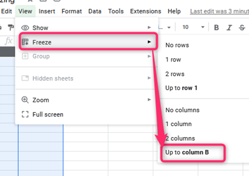
7. That’s all. The selected cells will be frozen.
To freeze more than two columns in Google Sheets
Steps:
1. Open Google Sheets
2. Open a new or existing Google sheets document you want to freeze its column.
3. Click on the column you want to freeze up to.
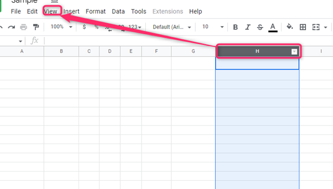
4. Then, click on the View tab on the menu. From the menu, hover the cursor over the Freeze button.
5. From the side-view menu, choose the Up to Column (the selected columns) button from the columns section.

6. That’s all. The selected cells will be frozen.
To unfreeze columns in Google Sheets
Steps:
1. Click on the View tab on the menu. From the menu, hover the cursor over the Freeze button.

2. From the side-view menu, choose the No column button.
To freeze columns in Excel
To freeze 2 columns
Steps to follow:
1. Open the Excel application.
2. Click on the third column.
When freezing columns in excel, we apply the freezing feature in the next column. If we want to freeze columns “A” and “B,” we will have to click on the third column, C.

3. Then, click on the View tab on the menu. Locate the Freeze Panes drop-down button.

4. From the menu, click on the Freeze Panes button. The two selected columns will be frozen.

The frozen column will be separated from other columns by a gray line that runs downwards. The columns on the left side of the line represent the frozen columns whereas those found on the right side are not frozen.
To freeze more than two columns in Excel
Steps:
1. Open the Excel application.
2. Click on the column next to the one you want to freeze.

3. Then, click on the View tab on the menu. Locate the Freeze Panes drop-down button.

4. From the menu, click on the Freeze Panes button. The two selected columns will be frozen.
To unfreeze cells
Steps to follow:
1. Open the Excel application.
2. Then, click on the View tab on the menu. Locate the Freeze Panes drop-down button.
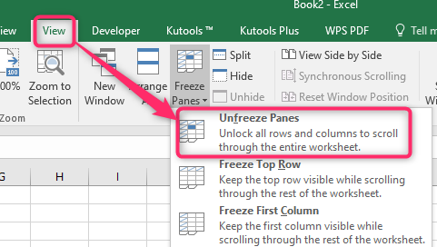
3. From the menu, click on the Unfreeze Panes button.