
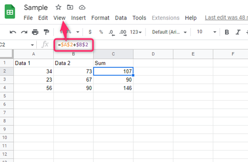
In Excel and Google Sheets, the formula is always displayed on the formula bar when you click the Cell that contains the formula. Thankfully, these two tools allow one to hide or show the formula. This post will discuss all the workarounds related to formulas.
To hide formulas in Google Sheets
Table of Contents
a) To hide formula in the cells
Here are the steps to follow:
1. Open the Google Sheets document that contains the formulas you want to hide.
2. Highlight the cells that contain the formula.
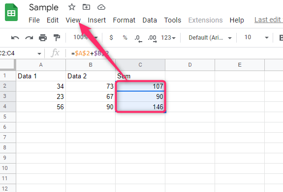
3. Click on the View tab on the toolbar.
4. Hover the cursor over the Show button, and uncheck the Formulas button.
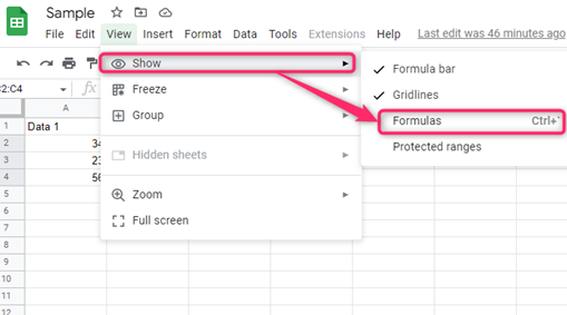
5. The formulas in the cells will be hidden.
b) To hide the Formula Bar
Here are the steps to follow:
1. Open the Google Sheets document that contains the formulas you want to hide.
2. Click on the View tab on the toolbar.
3. Hover the cursor over the Show button, and uncheck the Formula bar button.

4. The formula bar it will be hidden.
c) To hide formula using the protected sheet feature
Steps:
1. Highlight the cells you want to hide.
2. Right-click on the selected cells and hover the cursor over the View cell more actions button.
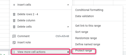
3. From the side-view pane, choose the Protect range button.
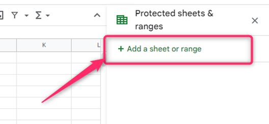
4. Click the Add a range or sheet button on the right pane.
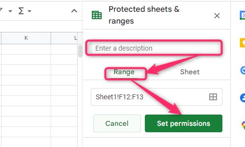
5. Then, enter the description of the Cell in the Description box. Then, click on the Set permissions button.
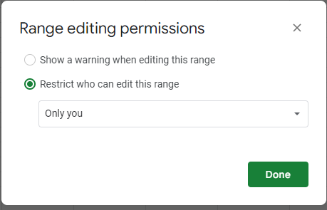
6. Choose who can edit the Cell from the dialogue box, and hit the Done button.
To hide formulas in Excel.
a) To hide formula in the cells
Three methods can be used:
Using the right-click tool
Steps:
1. Open the Excel document where you want to hide the formulas.
2. Highlight the cells that contain the cells you want to hide.
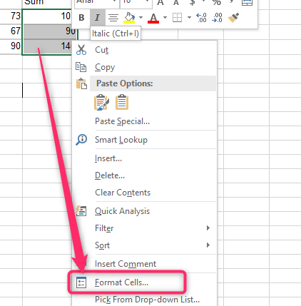
3. Right-click on the highlighted cells. From the menu, click the Format cells button.
4. From the format dialogue box, click on the Protection tab.
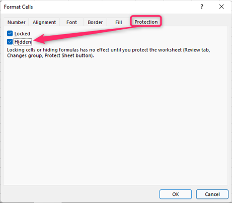
5. Check the hidden checkbox.
Using Number Dialogue launcher
Steps:
1. Open the Excel document where you want to hide the formulas.
2. Highlight the cells that contain the cells you want to hide.
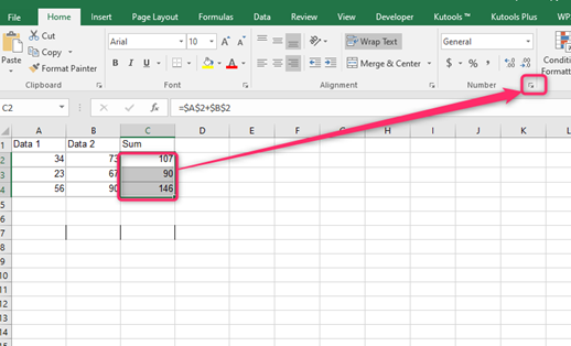
3. Click on the Home tab and locate the number dialogue launcher in the Number section.
4. From the format dialogue box, click on the Protection tab.

5. Check the Hidden checkbox.
Using the format tool
Steps:
1. Open the Excel document if you want to hide the formulas.
2. Highlight the cells that contain the cells you want to hide.
3. Click on the Home tab, and then locate Format drop-down button in the Cells section.
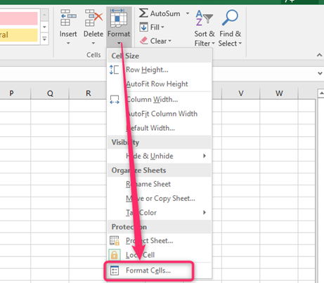
4. From the drop-down, choose the Format Cells button.
5. From the format dialogue box, click on the Protection tab.

6. Check the Hidden checkbox.
b) Using Protect sheet to hide the formula
Steps:
1. Open the Excel document if you want to hide the formulas.
2. Highlight the cells that contain the cells you want to hide.
3. Click on the Review tab and the Protect sheet button.
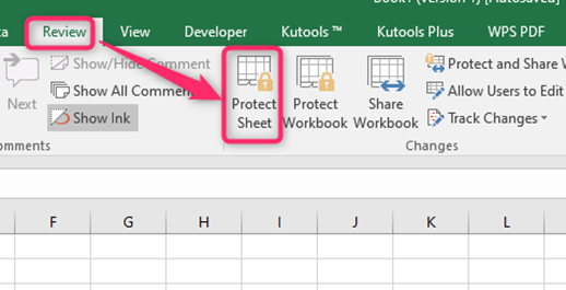
4. Type the password, and select the locking features you want.