

Google Sheets and Excel allow the user to check and know the position of a specific text or value within the dataset. Inbuilt functions are used to check the relative position of items in Google Sheets and Excel. This article will discuss how to match two columns in Google Sheets and Excel.
To match in Google Sheets
Table of Contents
Methods that can be used:
Using the Match function
Using the Vlookup formula
Conditional formatting tool
Using the Match function
Steps:
1. Visit the Google account and log in using your email detail (That is, https://www.google.com/account).
2. From the Google Apps, click on the Sheets icon and select the existing Sheet.

3. locate the columns you want to match. Click on the third column, and type the match function.
=MATCH (search_key, range, search_type)

4. Then, hit the Enter button.
Using the Vlookup function
Steps:
1. Visit the Google account and log in using your email detail (That is, https://www.google.com/account).

2. Locate the columns you want to match. Click on the third column, and type the =VLOOKUP(.
3. Enter the Search key and hit the comma button.
4. Select the range you want to apply the formula and hit the comma button. That is, =VLOOKUP( Search_key, range,

5. Finally, choose the Index and close the function. That is, =VLOOKUP( Search_key, range, index).
Conditional formatting tool
Steps:
1. Locate the columns you want to match
2. Highlight the whole dataset and click on the format tab in the menu.
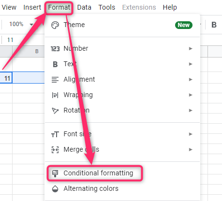
3. From the menu, choose the Conditional formatting button. A conditional formatting pane will open on the right side of the screen.
4. Choose the Custom formula if the button in the Format cell If section. In the value or formula section, type this formula =MATCH (search_key, range, search_type)

5. In the Apply range section, choose the two-column you want to match.
6. In the Formatting style section, choose the fill color, font color, and font format you want.
7. Finally, hit the Done button.
To match in Excel
Methods that are used:
Using the Match function
Using the Vlookup formula
Conditional formatting tool
Using the Match function
Here are the steps to follow:
1. Open the Excel application.
2. locate the columns you want to match. Click on the third column, and type the match function.
=MATCH (search_key, range, search_type)

3. Then, hit the Enter button
Conditional formatting tool
Steps:
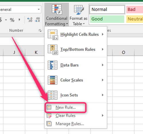
1. Highlight the two columns and click on the Home tab in the menu.
2. From the menu, click on the Conditional formatting drop-down button. Choose the New Rule button.
3. In the dialogue box, choose the Use a formula to determine which cell to format option. Enter this formula, ==MATCH (search_key, range, search_type)
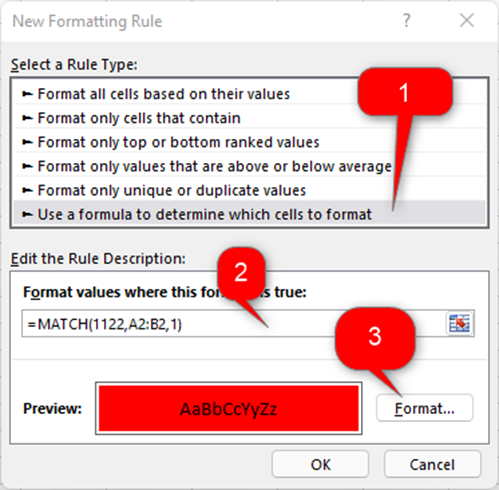
4. Click on the Format button and customize the formatting.
5. Finally, hit the Enter button.
Using the Vlookup function
Steps:
1. Locate the columns you want to match. Click on the third column, and type the =VLOOKUP(.
2. Enter the Search key and hit the comma button.
3. Select the range you want to apply the formula and hit the comma button. That is, =VLOOKUP( Search_key, range,
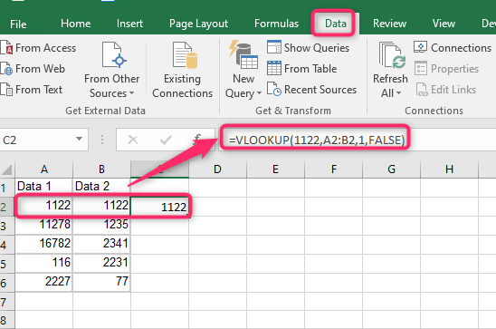
4. Finally, choose the Index and close the function. That is, =VLOOKUP( Search_key, range, index).