

In Google sheets, the columns are labeled using alphabetic letters, i.e., A-Z. These letters are frozen. Thus, they will always appear as you scroll down your document. You can’t rename them. However, Google sheet allows users to create names and freeze another row that can be used as the columns headers. This article shall discuss some of the common techniques used in naming the column.
Naming Column Headers
Table of Contents
If you want to name your column headers, follow these steps:
1. Open the Google sheet using the browser of your choice. That is, go to https://docs.google.com/ and log in using your email details.
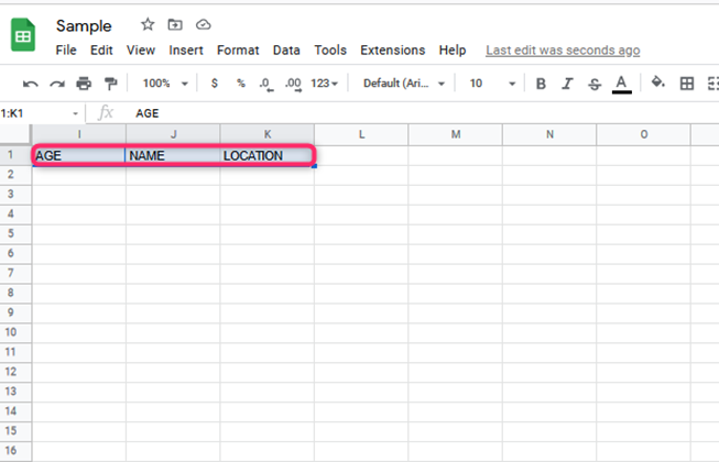
2. On a new document, select the top row. It is where you will add the column headers.
3. Click on the first cell within the first row. Enter the first header that will represent the dataset below that column.
4. Proceed and enter the header on the other cells of the first row.
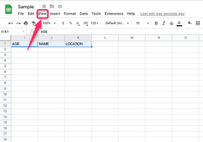
5. Now that you have the headers, you can freeze this row. To freeze the row that contains the headers, follow these steps:
- On the menu section, locate and click on the View option.
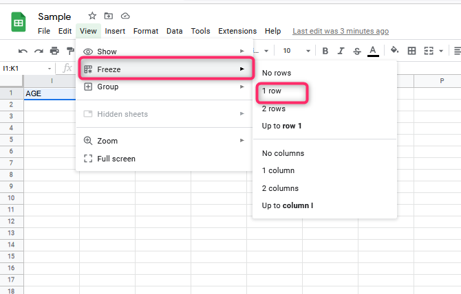
- On the drop-down menu, hover the mouse on top of the freeze button.

- Then, select either 1 row or up to row 1. When using the Up to row 1 option, you must highlight the top row first.
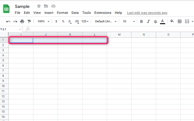
6. Your entire column header will have names and always appear as you scroll down the sheet.
One column header for many columns
Another way to name your column is by using one header in more than one column. Here are the steps to do so:
1. Open the Google sheet you are working on.
2. Then, highlight the cells of the top rows where you’ll place your header.
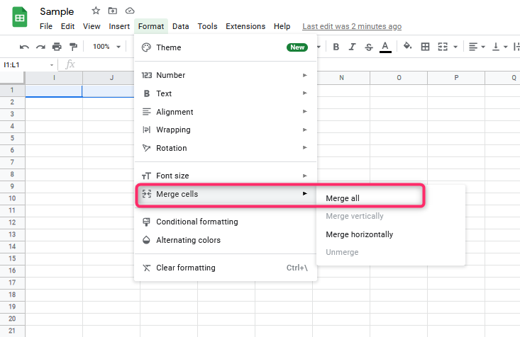
3. On the menu bar, click the Format tab. On the drop-down menu, hover your mouse on top of the merging cells button.

4. On the side-view menu, click the Merge all button.
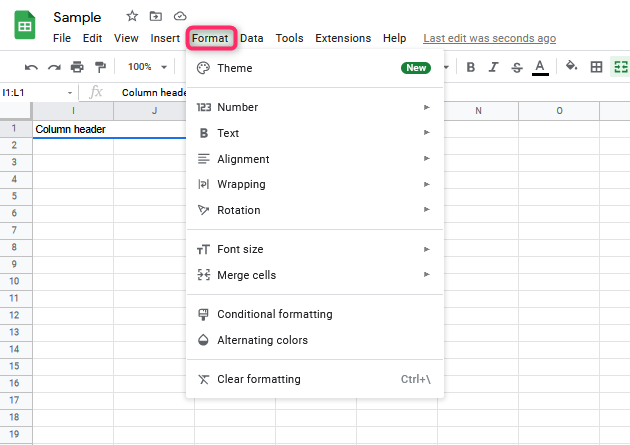
5. Go ahead and input your header on the merged cells.
To align the header, follow these:
- Highlight your column header and click the Format tab.
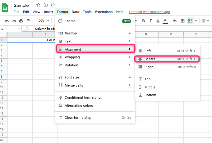
- Hover the cursor on top of the Alignment button and select center. Alternatively, you can use keyboard shortcuts. That is CTRL +SHIFT +E.
How to Name columns On Mobile Phone
Here are the steps to follow when using a mobile phone:
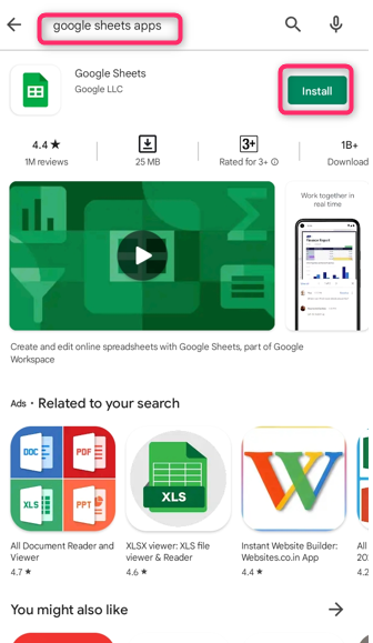
1. Download and install Google sheet App from the play store.
2. To open a new sheet, click the untitled spreadsheet.
3. On the top row, enter the names or titles of your column on those cells.

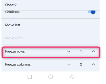
4. Then, click on the drop-down button located on the sheet name.

5. Locate the freeze rows button. Select the number of rows to be frozen. In this case, we will select one because we want to freeze the top row only.
You now have your column names.