
Google Sheets and Excel documents have gridlines that make up the cells. These two tools allow users to choose whether to print gridlines or not. While printing, the user can choose either to print gridlines or not. This post will discuss workarounds related to printing gridlines.
To print Gridlines in Google Sheets.
Table of Contents
To print gridlines in Google Sheets, you need to follow these steps:
1. Open the Google Sheets document where you want to add the gridlines. Make sure you are connected to the printer either wirelessly or wired.
2. Click on the File tab on the toolbar.

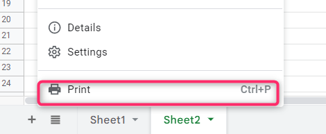
3. From the menu, click on the Print button. Alternatively, press the CTRL + P keys on your keyboard to open the print screen.

4. In the Print screen, click on the Formatting button.
5. In the formatting menu, check the Show gridlines checkbox.

To Print Gridlines in Excel
Similarly, Excel allows users to print gridlines in their documents. Here are the steps to do so:
1. Make sure you are connected to the printer, and then click on the File tab on the toolbar.

2. From the menu, click on the Print button. Alternatively, press the CTRL + P keys on your keyboard to open the print screen.
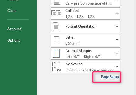
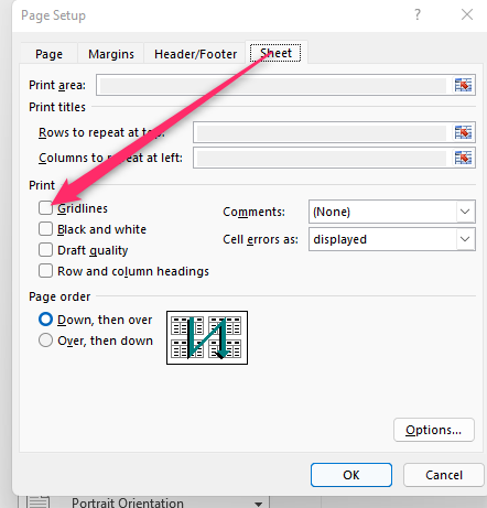
3. From the menu, click on the Page Setup button.
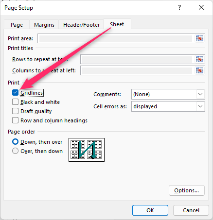
4. Click on the Sheet tab in the dialogue box, and then check the Gridlines button.
To hide Gridlines while printing.
a) To hide in Google Sheets
Steps to follow:
1. Open the Google Sheets document that you want to remove the gridlines.
2. Click on the File tab on the toolbar.

3. From the menu, click on the Print button. Alternatively, press the CTRL + P keys on your keyboard to open the print screen.
4. In the Print screen, click on the Formatting button.

5. In the formatting menu, uncheck the Show gridlines checkbox.
b) To hide in Excel
Steps to follow:
1. Open the Excel document in which you want to remove the gridlines.
2. Click on the File tab on the toolbar.

3. From the menu, click on the Print button. Alternatively, press the CTRL + P keys on your keyboard to open the print screen.
4. From the menu, click on the Page Setup button.

5. Click on the Sheet tab in the dialogue box, and then uncheck the Gridlines button.
6. Finally, click the Ok button.
To show gridlines in Worksheet
To show gridlines in Excel
Steps:
1. Open the Excel document in which you want to remove the gridlines.
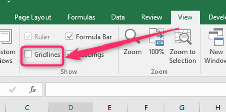
2. Click on the View tab on the toolbar.

3. Locate the Show section, and check the gridlines button.
To show gridlines in Google Sheets.
Steps:
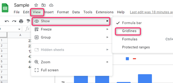
1. Open the Google Sheets document where you want to add the gridlines.
2. Click on the View tab on the toolbar.

3. Hover the cursor over the Show button, and check the Gridlines button.
4. That’s all.
To hide gridlines in Worksheet
a) Google Sheets
Steps:
1. Open the Google Sheets document that you want to remove the gridlines.
2. Click on the View tab on the toolbar.
3. Hover the cursor over the Show button, and uncheck the Gridlines button.
4. All the gridlines that will be removed from your document.
b) In Excel
Steps:
1. Open the Excel document in which you want to remove the gridlines.
2. Click on the View tab on the toolbar.
3. Locate the Show section, and uncheck the Gridlines button.
4. That’s all.