While working with Google Sheets and Excel, the cells may keep changing and moving as you work on the dataset. However, Google Sheets and Excel allows user to control the cell constant as they work efficiently. This article will discuss the ways to keep the cells steady.
To keep cell constant in Google Sheets
Table of Contents
Methods that can be used:
Keeping cell constant in the formula
Freezing the cell
Keeping cell constant in the formula
Here are the steps to follow:
1. Visit the Google account and log in using your email detail (That is, https://www.google.com/account).
2. From the Google Apps, click on the Sheets icon and select the existing Sheet.

3. Open the dataset that contains the formula you want to keep constant.
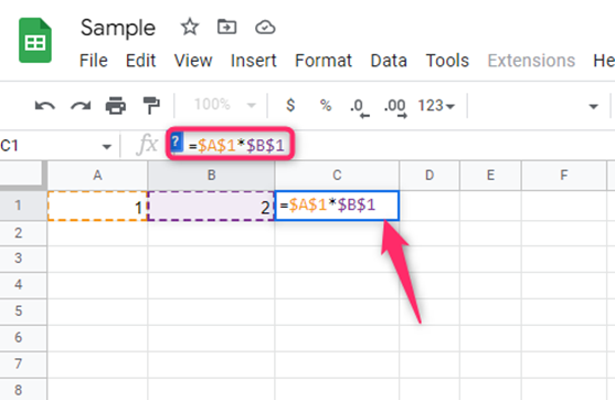
4. Click on the cell reference you want to keep constant and enter the Dollar sign before the column and the row ($A$2).

5. Alternatively, you can click on the F4 key to make the cell constant
Freezing the cell
Steps to follow:
1. Visit the Google account and log in using your email detail (That is, https://www.google.com/account).
2. Open a new or existing Google sheets document you want to freeze its column.
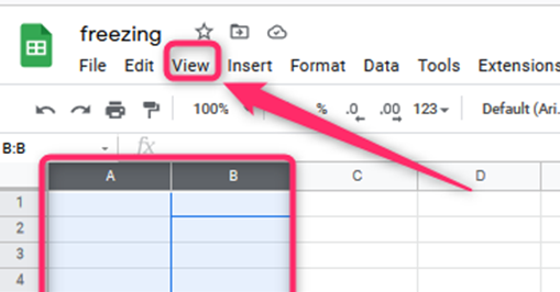
3. Highlight the two columns you want to freeze.

4. Then, click on the View tab on the menu. From the menu, hover the cursor over the Freeze button.

5. From the side-view menu, choose the Up to Column (the selected columns) button from the columns section.

6. That’s all. The selected cells will be frozen.
To keep cell constant in Excel
Keeping cell constant in the formula
Here are the steps to follow:
1. Open the Excel application.
2. Open the dataset that contains the formula you want to keep constant.
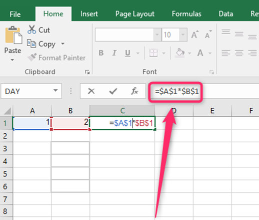
3. Click on the cell reference you want to keep constant and enter the Dollar sign before the column and the row ($A$2).

4. Alternatively, you can click on the F4 key to make the cell constant
Freezing tool
Steps to follow:
1. Open the Excel application.
2. Click on the third column.
When freezing columns in excel, we apply the freezing feature in the next column. If we want to freeze columns “A” and “B,” we must click on the third Column, C.

3. Then, click on the View tab on the menu. Locate the Freeze Panes drop-down button.

4. From the menu, click on the Freeze Panes button. The two selected Columns will be frozen.

To freeze more than two columns in Excel
Steps:
1. Open the Excel application.
2. Click on the column next to the one you want to freeze.

3. Then, click on the View tab on the menu. Locate the Freeze Panes drop-down button.

4. From the menu, click on the Freeze Panes button. The two selected columns will be frozen.
To unfreeze cells
Steps to follow:
1. Open the Excel application.
2. Then, click on the View tab on the menu. Locate the Freeze Panes drop-down button.

3. From the menu, click on the Unfreeze Panes button.

