When using Google Sheets, it is obvious that you will have to use dates. You can format these dates for your preference and convenience. It is important to note that Google Sheets stores all its dates as integer numbers, not as sequences of the day, month, or year as it was in Excel. Google also stores dates before December 31, 1899, as negative numbers.
How to change the date format in Google Sheets to another Locale
Table of Contents
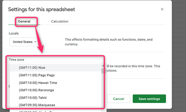
The Locale presets your Google Sheets date format based on your region. For example, if you are in the United States, 06-Aug-2020 will be written as 8/6/2020. If the file was made in another country, you could change it according to your Locale. It is vital to know that Locale does not change the language of your Google Sheets. Use the following method
1. Open File in the Google Sheets menu

2. Go to the General tab to find Locale, thus picking up the desired location from the list of choices given

3. It is also important to specify the time of your zone.
The Default Sheets’s date format
Use the following method;
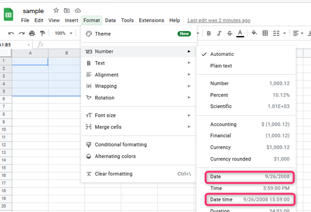
1. Highlight the “cells” that you need to format

2. Open Format
3. Click on Number in the spreadsheet menu

4. Choose on Date /Date time

In this regard, integers will turn to the format you will recognize. For example, the format can be as day/ month/ year.
The Custom Date formats
You can improvise the dates in Google Sheets if you don’t like the one offered by Google Sheets. You can access the Custom Date formats by following the method below;
1. Open Format
2. Click on Number

3. Choose More Format
4. Click on More date and time formats

The window that appears has different custom date formats available. The system will apply whichever one that you choose and apply. You can also create your custom date format using the following;
1. Highlight the cells that you want to format
2. Open Format
3. Click on Number

4. Go to More Formats
5. Click on date and time formats

6. Position the cursor in the field that has date units and then delete everything using Backspace and Delete Keys

7. Use your mouse to select the arrow at the right of the field and then select the unit you would like to have.
8. Click on the units so that you can adjust the units with double arrows so that they can exactly display the value

9. Click on Apply

If you want to change the “format of the date” in each cell, follow the following easy steps;
1. Open Format, then click on Number
2. Go to More Formats
3. Choose More Date and Time Formats

4. Choose the format you want to apply

5. If you want to apply the specific format to all cells, select the row number or “column” that you need to apply this
It thus becomes easy to switch update settings to personalize your spreadsheet.

