

We have multiple ways to turn negative numbers red in Google sheets. The red color will enable negative numbers to stand out when analyzing data. You can use conditional formatting or custom number formatting to highlight negative numbers in red. Conditional formatting will highlight the whole cell, while custom numbers will only highlight the numbers. Further, people love red because it is a shouting color, but you can use any color. We will use red as it is the default color used around the globe.
Use of Conditional Formatting
Table of Contents
The feature allows you to color a cell based on the value within the cell. The procedure will turn negative numbers red while others will remain the same.
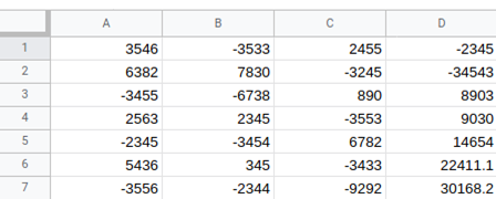
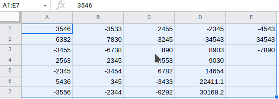
1. Open Google Sheets on your computer and open the file you want to have these changes done to it. When you open the file, you will notice that negative numbers are very hard to spot in the large dataset.
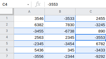
2. Select the cells you want to highlight in red. (The cells with negative numbers only.) Click format in the google sheet tab.
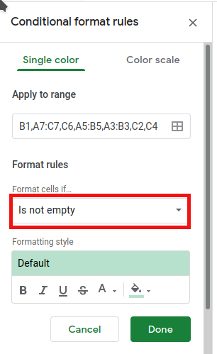
3. In the prompt menu, select conditional formatting; this will open the conditional formatting rules panes on the right.

4. Click on the format cells if drop-down.
5. Click on the less than an option. ( scroll down to see the option).
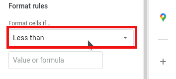
6. In the value or format, place 0.

7. Select the color with which you want to highlight the cell. (Go to the formatting style)
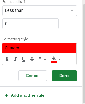
8. Click done.

The steps above will highlight all cells with numbers less than 0 red. Less than 0 is any number with a negative sign. Conditional formatting is dynamic; any change you make to your sheet formatting will be updated automatically.
Using custom number formatting
Conditional formatting is an easy way to turn a negative number red. It happens by changing the custom number formatting. It will ask you to specify positive, negative, zero, and text values.
1. Select the whole dataset.
2. Click format in the menu.

3. Go to the number option and hover the cursor over it. You will see additional options for you.

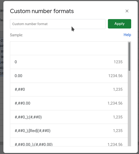
4. Click custom number format, and do the following. (some time back, excel had other additional information under custom number form.)

5. Click the custom number format. It will open a custom dialog box.
6. Go to the format field, enter this: General;[RED]General; General;@
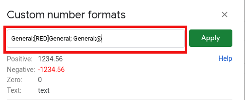
7. Click the apply button.

All negative numbers will turn red.
Note: In conditional formatting, the cell will be highlighted in red, but in custom number formatting, the color of the “value” will be red.
Google sheet is amazing; it will allow you to analyze data easily and fast. Looking for a negative number within a google spreadsheet will be cumbersome. Time-consuming, doing this will enable you to see negative numbers quickly. Careful you don’t distort your data or information.