Google Sheets has four ways to join texts. You can use the functions JOIN, TECTJOIN, CONCATENATE, or Ampersand.
Using the JOIN function
Table of Contents
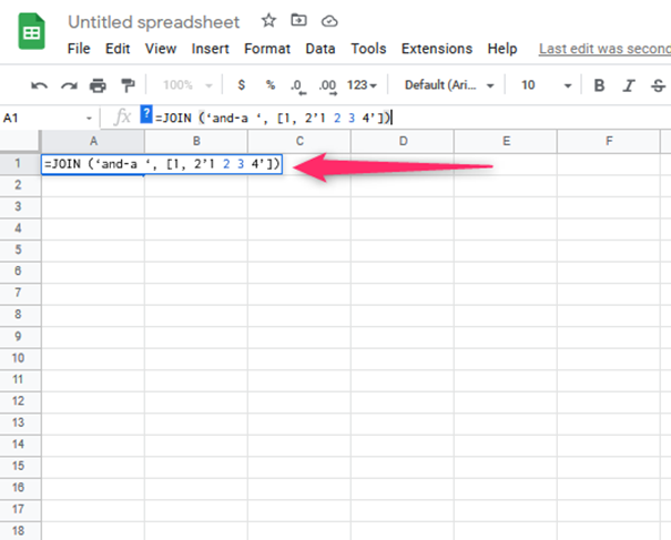
The Join function joins one or two-dimensional array elements while using a specified delimiter. You can use the samples below;
JOIN (‘and-a, ‘[1, 2’1 2 3 4’])

JOIN (“,”, [1, 2, 3], [4; 5; 6])
JOIN (“-, ” A1:A100)
The joining syntax is
JOIN (delimiter, value_or_array1, [value_or_array2,])

The delimiter character is placed between each value. It may be specified with a blank.
The value_or_array1,]) are values to be appended using the delimiter character.
The value_or_array2 is an optional character and is just an additional value that is appended by the delimiter feature.
There are occasions when you are not supposed to use the JOIN function in Google Sheets. One of them is when you want to combine two tables with different numbers of columns. The JOIN function will not include the columns from the first table if the number of columns in the two tables does not match. You should not use the JOIN function when trying to merge data from two different sheets. In this case, the JOIN function will not be able to combine the data if the sheets have different column headers.
Similar formulae to JOIN Goole Sheets
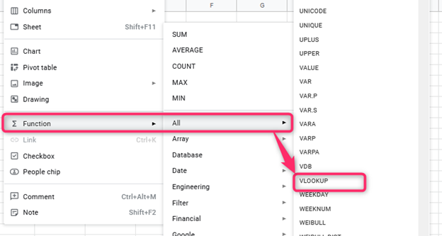
Similar formulae to JOIN in Google sheets include the VLOOKUP and CONCATENATE functions. VLOOKUP allows you to look up data based on a particular value in a table. The CONCATENATE allows the user to combine text from multiple cells into one particular cell. The AVERAGE is another function that allows the user to calculate the average of the number set you are using.

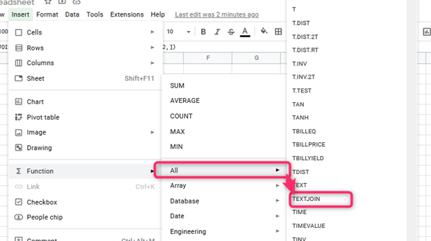
Using the TEXTJOIN Function in Google Sheets
This function joins texts in multiple arrays where a delimiter can also separate the joined texts. The syntax that can be used is; TEXTJOIN (delimiter, ignore_empty, text1, [text2….])

The delimiter is just a character in between the strings. The ignore_empty string controls blank cells in the range you have selected. The text1 contains the text to be joined or the text itself.
Using the formula to
1. Join tables
In this case, the formula is used to join two tables to produce similar results to LEFT JOIN n SQL. For every row of data on the left (table A), you are given a matching row in table b. You will get an empty cell when the row in table a does not match the row in table B.
2. For Multiple criteria
The VLOOKUP function is the standard way to match up data in Google Sheets. This function specifies a key from table A, such as a cell-like A2. VLOOKUP will look for the first value that matches the first column in table B.

Remember that columns in the lookup range can be arranged in any order. For the VLOOKUP function, the key in the second table should always be the first column of the table.

