When we are using excel or google spreadsheets sometimes we enter a lot of information or simply large data in one cell which. This makes the data force the cell to extrapolate and therefore seems to continue past its column if the adjacent column is empty. If the column adjacent has some content, then the data in the cell is cut-off and so only data within the cell’s default size is displayed.
To avoid this, we can wrap the text and make it display on multiple lines inside the same cell. Although this pushes the cell and its row to increase in height, it is better because it makes reading the content easier as all the content in the cell is visible. When you print the spreadsheet without wrapping the data, the whole data will not appear. Instead, the data that is visible within the cell’s default size will be seen. It also helps to keep the whole column width uniform throughout the whole spreadsheet.
The following steps show how we can wrap data in a cell in both google sheets and excel.
In Google Sheets;
Table of Contents
1. Open Google Sheets from a web browser.
2. Select the cells, columns, or rows whose contents you want to keep in a single cell. (wrap).

If you want to select multiple cells, hold CTRL on your keyboard and click the cells you want to highlight.
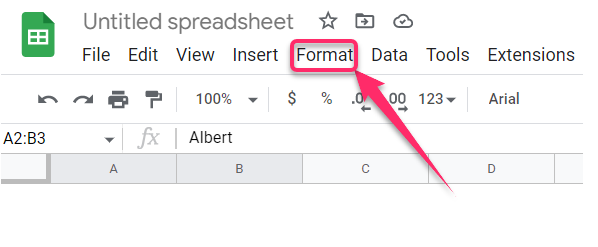
3. Click the Format tab from the menu bar.

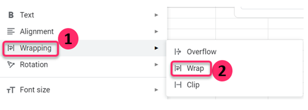
4. From the options that pop up click, Wrapping, then Wrap.

All the content in the cell will be wrapped.

In Excel;
1. Open Microsoft excel from your computer applications and the spreadsheet with the cell you want to wrap.
2. Select the cell that you want to wrap its content.

If you want to select multiple cells, then hold CTRL while clicking the cells you wish to highlight on your keyboard.
3. From the menu bar click the Home tab.

4. From the options provided in the Alignment group click Wrap Text.


