
While working with Google Sheets and Excel, formulas are common. These two tools allow the user to lock the formula in the locked cells. This post will discuss ways of locking formulas in Google Sheets and Excel.
To lock a formula in Google Sheets
Table of Contents
a) To lock cells in the formula
Cells in the formula are the cell references that directly affect the formula. For example, if the formula is =A2+A3, the cells in that formula are A2 and A3.
Here is the step to lock cells in the formula:
1. Open the Google Sheets document that contains the formula you want to lock.
2. Click on the Cell that contains the formula.
3. On the formula bar, locate the formula.
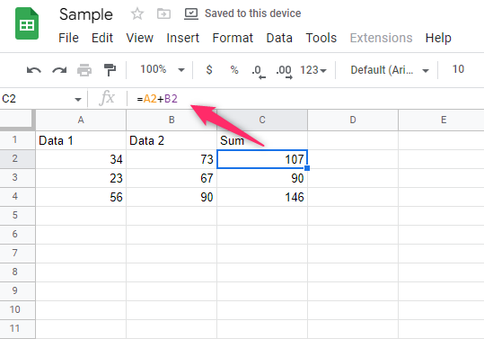
4. To lock the formula cells, add the Dollar sign between the column index and the row index. For example, =$A$2+$A$3

5. Finally, click on the Enter button.
b) To lock cells with the formula
Cells with the formula are the cells that hold the formula. Below are the steps to lock them:
1. Highlight the cells you want to lock.
2. Right-click on the selected cells and hover the cursor over the View cell more actions button.

3. From the side-view pane, choose the Protect range button.
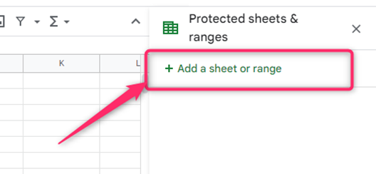
4. Click the Add a range or sheet button on the right pane.
5. Then, enter the description of the Cell in the Description box. Then, click on the Set permissions button.

6. Choose who can edit the Cell from the dialogue box, and hit the Done button.

c) To lock a single Cell with the formula
Steps:
1. Locate and click on the Cell you want to lock.
2. Right-click on the selected Cell and hover the cursors over the View cell more actions button.

3. From the side-view pane, choose the Protect range button.

4. Click the Add a range or sheet button on the right pane. Then, enter the description of the Cell in the Description box.

5. Then, click on the Set permissions button. Choose who can edit the Cell from the dialogue box and hit the Done button.

To lock a formula in Excel
a) To lock cells in the formula
Steps:
1. Open the Excel document.
2. Click on the Cell that contains the formula.
3. On the formula bar, locate the formula.

4. To lock the formula cells, add the Dollar sign between the column index and the row index. For example, =$A$2+$A$3

5. Finally, click on the Enter button.
b) To lock a single cell
Steps to follow:
1. Open the Excel application.
2. Click on the Cell you want to lock.
3. Click on the Home tab, hit the Format Cells drop-down button, and choose the Lock Cell option.

c) To lock multiple cells with a formula
Steps to follow:
1. Open the Excel application.
2. Highlight the cells that have the formula.
3. Right-click and choose the Format Cells option.

4. From the dialogue box, click on the Protection tab.
5. Check the Locked checkbox.

d) To lock the Entire Sheet
Steps to follow:
1. Open the Excel application.
2. Click on the Cell you want to lock.
3. Click on the Home tab, hit the Format Cells drop-down button, and choose the Protect Sheet option.

4. Enter the locking password in the password section.
5. Using the Checkbox, check or uncheck the checkboxes in the Allow all users of this worksheet section.
