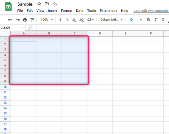
Create a conditional formatting rule
Steps to apply conditional formating
Table of Contents
1. Select the cell range.

2. Click the format on the menu bar.
3. Select conditional formatting.

4. Under the format, there are various options: bold, italic, underline, font size, align, and others. Don’t select any of the options.
5. Since the conditional format rule appears and already the new rule has been commerce, select the conditions for the formatting to the appearance.

6. The formatting that will appear should be customized to meet the conditions.
7. Click OK and done.

The rule is already saved at this point.
The conditions and their descriptions
Under this, the user should know the needed conditions to apply the formatting appropriately. They show what the specified condition means in the formatting conditions.
Is empty
It applies formatting for empty cells.
Is not empty
It applies to the format for the cells that are not empty.
“Text contains”
It applies “formatting for cells” that have specified text.
“Text does not contain.”
It applies “formatting for cells” that don’t have a specified text.

Text starts with
Applies formatting for cells that start with specified text.
Text ends with
Applies formatting for cells that end with specified text.
Text is exactly
It applies formatting for cells that are exactly the specified text.
Date is
It applies to formatting for cells with dates matching a specified date.
Date is before
It applies formatting for cells with dates that are before a specified date.
Date is after
It applies formatting for cells with dates that are after a specified date.

Greater than
It applies to formatting for cells with values greater than that specified value.
Greater than or equal to
It applies formatting for cells with values greater than or equal to a specified value.
Less than
It applies to formatting for cells with less than that specified value.
Less than or equal to
It applies formatting for cells with values less than or equal to a specified value.
Is equal to
It applies to the formatting for cells with values equal to that specified value.
Is not equal to
It applies formatting for cells with values not equal to that “specified value.”
“Is between”
It applies “formatting for cells” with values between two specified values.
“Is not between.”
It applies to formatting cells with values, not between two specified values.
Custom formula is
It applies formatting for cells with custom formulas.

How to delete a conditional formatting rule
If you need to delete the already set rule, check this
1. Select a cell within the conditional formatting range.

2. Under the conditional format rule, open it.
3. Click the option of the remove rule button.

The rule is deleted.
These conditions should be applied appropriately. Deleting the conditional formatting in your computer avoids confusion within the cells that are yet to be opened. If not deleted, it might cause inconvenience during other works like typesetting.

